rxode2 2.0.9/2.0.10
By Matthew Fidler in rxode2
October 19, 2022
rxode2 2.0.9 has been released, and rxode2 2.0.10 will be released
soon! I want to personally thank all those who have submitted issues,
and helped with the development. Without the support rxode2
wouldn’t be the tool it is today.
This is the first CRAN-visible release since rxode2 2.0.7 and I
would like to highlight a few new interesting features:
‘rxode2’ can now have more flexible model functions
The key features are:
- You do not need an
ini()block any longer - You do not need to specify an endpoint either with
~
For example, this model is perfectly reasonable in rxode2:
set.seed(42)
rxSetSeed(42) # for parallel random number generator

one.compartment <- function() {
  model({
    ka <- exp(tka + eta.ka)
    cl <- exp(tcl + eta.cl)
    v <- exp(tv + eta.v)
    d / dt(depot) <- -ka * depot
    d / dt(center) <- ka * depot - cl / v * center
    F(depot) <- 3
    cp <- center / v
  })
}

m <- one.compartment()

m
## ── rxode2-based free-form 2-cmt ODE model ──────────────────────────────────────────
##
## States ($state or $stateDf):
## Compartment Number Compartment Name
## 1 1 depot
## 2 2 center
## ── Model (Normalized Syntax): ──
## function() {
## model({
## ka <- exp(tka + eta.ka)
## cl <- exp(tcl + eta.cl)
## v <- exp(tv + eta.v)
## d/dt(depot) <- -ka * depot
## d/dt(center) <- ka * depot - cl/v * center
## F(depot) <- 3
## cp <- center/v
## })
## }# When solving you will have to manually supply the parameters
theta <- c(tka = 0.45, tcl = 1,tv = 3.45)
omega <- lotri({eta.ka ~ 0.6
eta.cl ~ 0.3
eta.v ~ 0.1
})
# Create an event table
et <- et(amt=300) %>%
et(0,24, by=2) %>%
et(id=1:12)
# simulate directly from the model
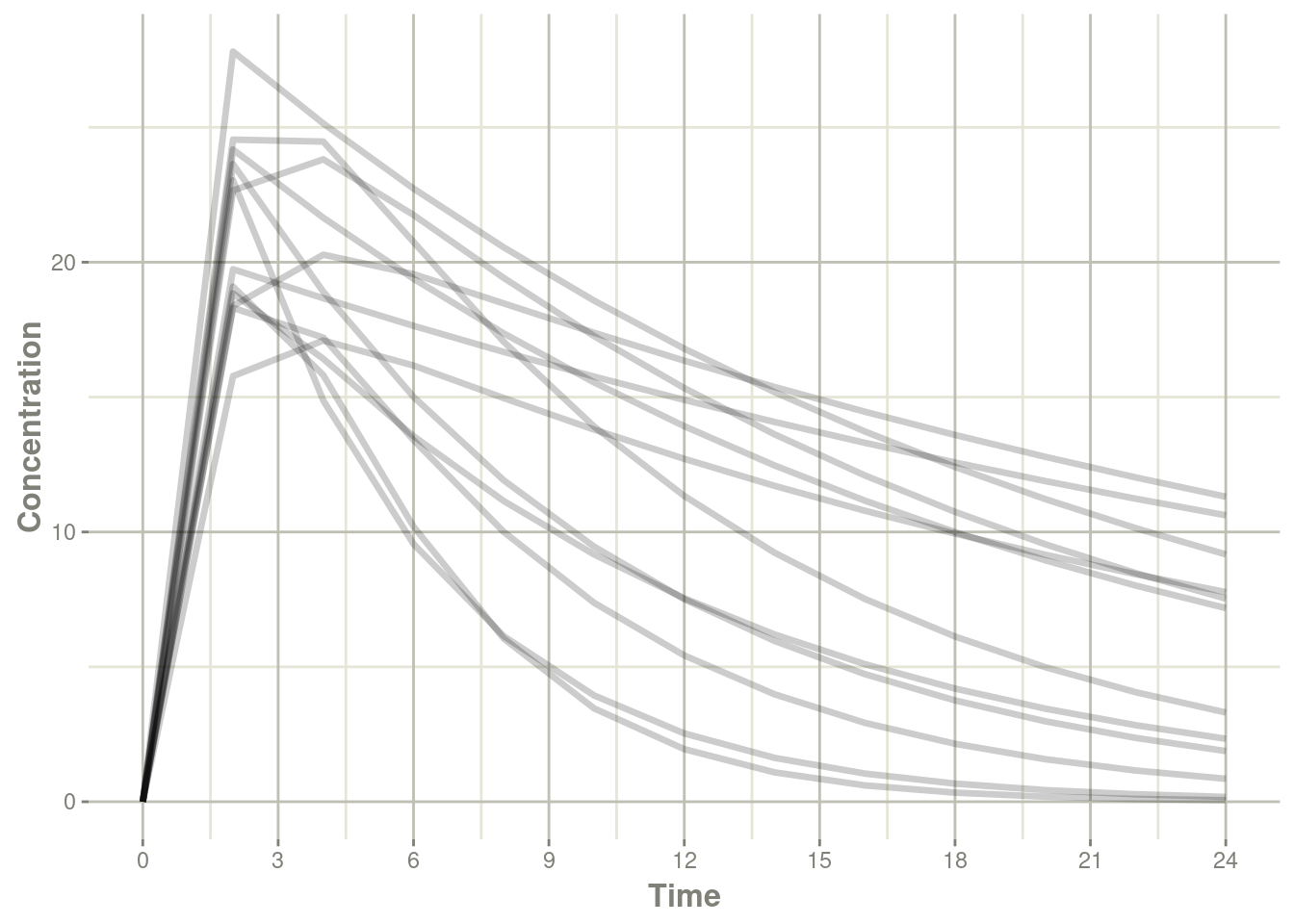
s <- rxSolve(m, et, theta, omega=omega)## → creating rxode2 include directory## → getting R compile options## → precompiling headers## ✔ donelibrary(ggplot2 )
plot(s, cp) + ylab("Concentration")
You can now pipe omega matrices to set initial values
For example, using the above model you could the omega initial values:
m2 <- m %>%
  ini(omega)
## ℹ promote `eta.ka` to between subject variability with initial estimate 0.6## ℹ change initial estimate of `eta.ka` to `0.6`## ℹ promote `eta.cl` to between subject variability with initial estimate 0.3## ℹ change initial estimate of `eta.cl` to `0.3`## ℹ promote `eta.v` to between subject variability with initial estimate 0.1## ℹ change initial estimate of `eta.v` to `0.1`print(m2)## ── rxode2-based free-form 2-cmt ODE model ──────────────────────────────────────────
## ── Initalization: ──
##
## Omega ($omega):
## eta.ka eta.cl eta.v
## eta.ka 0.6 0.0 0.0
## eta.cl 0.0 0.3 0.0
## eta.v 0.0 0.0 0.1
##
## States ($state or $stateDf):
## Compartment Number Compartment Name
## 1 1 depot
## 2 2 center
## ── Model (Normalized Syntax): ──
## function() {
## ini({
## eta.ka ~ 0.6
## eta.cl ~ 0.3
## eta.v ~ 0.1
## })
## model({
## ka <- exp(tka + eta.ka)
## cl <- exp(tcl + eta.cl)
## v <- exp(tv + eta.v)
## d/dt(depot) <- -ka * depot
## d/dt(center) <- ka * depot - cl/v * center
## F(depot) <- 3
## cp <- center/v
## })
## }# notice that the model now includes an `ini({})` block
# If you pipe the theta values, you can get a full model:
m2 <- m2 %>% ini(tka = 0.45, tcl = 1,tv = 3.45)## ℹ promote `tka` to population parameter with initial estimate 0.45## ℹ change initial estimate of `tka` to `0.45`## ℹ promote `tcl` to population parameter with initial estimate 1## ℹ change initial estimate of `tcl` to `1`## ℹ promote `tv` to population parameter with initial estimate 3.45## ℹ change initial estimate of `tv` to `3.45`print(m2)## ── rxode2-based free-form 2-cmt ODE model ──────────────────────────────────────────
## ── Initalization: ──
## Fixed Effects ($theta):
## tka tcl tv
## 0.45 1.00 3.45
##
## Omega ($omega):
## eta.ka eta.cl eta.v
## eta.ka 0.6 0.0 0.0
## eta.cl 0.0 0.3 0.0
## eta.v 0.0 0.0 0.1
##
## States ($state or $stateDf):
## Compartment Number Compartment Name
## 1 1 depot
## 2 2 center
## ── Model (Normalized Syntax): ──
## function() {
## ini({
## tka <- 0.45
## tcl <- 1
## tv <- 3.45
## eta.ka ~ 0.6
## eta.cl ~ 0.3
## eta.v ~ 0.1
## })
## model({
## ka <- exp(tka + eta.ka)
## cl <- exp(tcl + eta.cl)
## v <- exp(tv + eta.v)
## d/dt(depot) <- -ka * depot
## d/dt(center) <- ka * depot - cl/v * center
## F(depot) <- 3
## cp <- center/v
## })
## }# Which of course still allows simple solving:
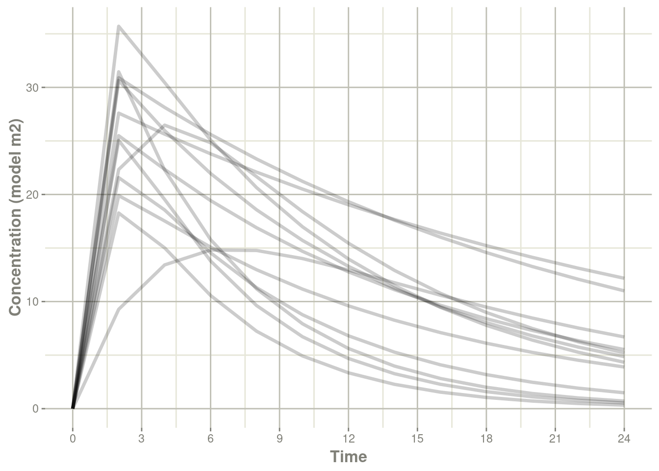
s <- rxSolve(m2, et)
plot(s, cp) + ylab("Concentration (model m2)") ## Piping classic
 rxode2 models
With the above flexibility, this release also allows piping of classic
rxode2 models:
For example:
rx <-  rxode2({
  ka <- exp(tka + eta.ka)
  cl <- exp(tcl + eta.cl)
  v <- exp(tv + eta.v)
  d / dt(depot) <- -ka * depot
  d / dt(center) <- ka * depot - cl / v * center
  F(depot) <- 3
  cp <- center / v
})

print(rx)
## rxode2 2.0.10 model named rx_3c919cdfd78bcd515c59521974200beb model (✔ ready).
## $state: depot, center
## $params: tka, eta.ka, tcl, eta.cl, tv, eta.v
## $lhs: ka, cl, v, cpm3 <- as.function(rx) %>%
ini(omega) %>%
ini(tka = 0.45, tcl = 1,tv = 3.45)## ℹ parameter labels from comments are typically ignored in non-interactive mode## ℹ Need to run with the source intact to parse comments## ℹ promote `eta.ka` to between subject variability with initial estimate 0.6## ℹ change initial estimate of `eta.ka` to `0.6`## ℹ promote `eta.cl` to between subject variability with initial estimate 0.3## ℹ change initial estimate of `eta.cl` to `0.3`## ℹ promote `eta.v` to between subject variability with initial estimate 0.1## ℹ change initial estimate of `eta.v` to `0.1`## ℹ promote `tka` to population parameter with initial estimate 0.45## ℹ change initial estimate of `tka` to `0.45`## ℹ promote `tcl` to population parameter with initial estimate 1## ℹ change initial estimate of `tcl` to `1`## ℹ promote `tv` to population parameter with initial estimate 3.45## ℹ change initial estimate of `tv` to `3.45`print(m3)## ── rxode2-based free-form 2-cmt ODE model ──────────────────────────────────────────
## ── Initalization: ──
## Fixed Effects ($theta):
## tka tcl tv
## 0.45 1.00 3.45
##
## Omega ($omega):
## eta.ka eta.cl eta.v
## eta.ka 0.6 0.0 0.0
## eta.cl 0.0 0.3 0.0
## eta.v 0.0 0.0 0.1
##
## States ($state or $stateDf):
## Compartment Number Compartment Name
## 1 1 depot
## 2 2 center
## ── Model (Normalized Syntax): ──
## function() {
## ini({
## tka <- 0.45
## tcl <- 1
## tv <- 3.45
## eta.ka ~ 0.6
## eta.cl ~ 0.3
## eta.v ~ 0.1
## })
## model({
## ka = exp(tka + eta.ka)
## cl = exp(tcl + eta.cl)
## v = exp(tv + eta.v)
## d/dt(depot) = -ka * depot
## d/dt(center) = ka * depot - cl/v * center
## f(depot) = 3
## cp = center/v
## })
## }Note the use of as.function() here, though it may not always be required in the future.
Why are there more dependencies for rxode2?
CRAN had requested that we reduce the compile time for ‘rxode2’ to remain on CRAN. This effectively was requesting the compile be split out to separate packages.
Note, now the packages that rxode2 depend on are:
rxode2parsewhich is the parsing of the rxode2 low level language to C (and includes some solved linear compartment code at the moment)rxode2randomwhich has the parallel safe random number generation routines, and some other random number generating functions likecvPost()rxode2llwhich includes the new likelihood functions supported in this release (which will add generalized likelihood estimation innlmixr2)rxode2etwhich therxode2event table functionet(), split off
What about when CRAN is out of sync (or temporarily dropped the packages)
Because the dependencies of ‘nlmixr2’ and ‘rxode2’ are currently a binary dependency of each other, if they were not compiled together they will not work together. You may get issues like “This was compiled against a different version of PACKAGE” when trying to load the package.
One approach is to use the r-universe to install the development version everything, that is:
install.packages(c("dparser", "rxode2ll", "rxode2parse",
                   "rxode2random", "rxode2et", "symengine", "rxode2",
                   "nlmixr2est", "nlmixr2extra",  "nlmixr2plot",
                   "nlmixr2"),
                 repos=c(nlmixr2="https://nlmixr2.r-universe.dev",
                         symengine="https://symengine.r-universe.dev",
                         CRAN="https://cloud.r-project.org"))
I would only suggest this if CRAN doesn’t seem to be working for your setup.
Full changes from 2.0.7
rxode2 2.0.10
Time invariant covariates can now contain ‘NA’ values.
When a column has ‘NA’ for the entire id, now ‘rxode2’ warns about both the id and column instead of just the id.
To fix some CRAN issues in ‘nlmixr2est’, make the version dependency explicit.
rxode2 2.0.9
Remove log likelihoods from
rxode2to reduce compilation time and increase maintainability ofrxode2. They were transferred to ‘rxode2ll’ (requested by CRAN).Remove the parsing from
rxode2and solved linear compartment code and move torxode2parseto reduce the compilation time (as requested by CRAN).Remove the random number generation from
rxode2and move torxode2randomto reduce the compilation time (as requested by CRAN).Remove the event table translation and generation from
rxode2and move torxode2etto reduce the compilation time (as requested by CRAN).Change the
rxode2ui object so it is a compressed, serialized object by default. This could reduce theC stack sizeproblem that occurs with too many environments in R.Warn when ignoring items during simulations
Export a method to change
rxode2solve methods into internal integersBug fix for time invariant covariates identified as time variant covariate when the individual’s time starts after
0.
rxode2 2.0.8
Breaking changes
rxgammanow only allows arateinput. This aligns with the internalrxode2version ofrxgammaand clarifies how this will be used. It is also aligned with thellikGammafunction used for generalized likelihood estimation.ui
cauchysimulations now follow the ui fornormalandtdistributions, which means you can combine with transformations. This is because thecauchyis atdistribution with one degree of freedom.ui
dnorm()andnorm()are no longer equivalent toadd(). Now it allows you to use the loglikllikNorm()instead of the standardnlmixr2style focei likelihood. This is done by addingdnorm()at the end of the line. It also meansdnorm()now doesn’t take any arguments.Vandercorput normal removed (non-random number generator)
New features
Allow models in the
nlmixr2form without anini({})blockAllow model piping of an omega matrix by
f %>% ini(omegaMatrix)Standard models created with
rxode2()can no be piped into a model functionFamilies of log-likelihood were added to
rxode2so that mixed likelihood nonlinear mixed effects models may be specified and run.The memory footprint of a
rxode2solving has been reducedPiping now allow named strings (issue #249)
Bug fixes
rxode2’s symengine would convertsqrt(2)toM_SQRT_2when it should beM_SQRT2. This has been fixed; it was most noticeable in nlmixr2 log-likelihood estimation methodsrxode2treatsDVas a non-covariate withetTran(last time it would duplicate if it is in the model). This is most noticeable in the nlmixr2 log-likelihood estimation methods.
New features
A new flag (
rxFlag) has been created to tell you where in therxode2solving process you are. This is useful for debugging. If outputting this variable it will always be11or calculating the left handed equations. If you are using in conjunction with theprintf()methods, it is a double variable and should be formatted with"%f".An additional option of
fullPrinthas been added torxode2()which allowsrprintf()to be used in almost all ofrxode2()steps (inductive linearization and matrix exponential are the exception here) instead of just the integrationddtstep. It defaults toFALSE.